


Written by: ck.eth
Compiled by: Lylia, Antalpha Labs
This is the fifth part of the original six-part series, which continues to introduce how options are combined with positions, and requires a certain understanding of the position strategies described earlier in the series. In order to allow more people to access and understand useful information about Uniswap V3, we translated the series of articles to give Chinese readers a deeper understanding of the Uniswap v3 mechanism and investment strategy selection. While reading this translation, you can always refer to the original article for more detailed information.
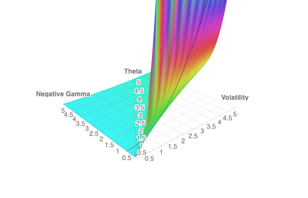
Nonlinearity / Theta-Gamma Volatility of Uniswap Return Convexity Risk. https://www.math3d.org/WvsEXvTWD
in short:
Demonstrated Greek solution for Uniswap v2 and v3
A solution for hedging Asian, European, and Bachelier options using Uniswapv3 is provided in the interactive desmos paper.
Demonstrated the use of desmos for LP hedging accumulation strategies.
The history and alternative derivations leading to LVR are explained.
Greeks - Uniswap v2
Rather than allocating 100% to the LP position, a partial allocation to asset X and the remainder to short asset X reduces but does not eliminate divergence losses. The result is a shift in the payoff structure from a cliff to a hill, as Guillaume Lambert shows: The Greeks tell one about the sensitivity of the value of the LP position with respect to another variable, such as time, volatility, and interest rates. We introduced Delta and Gamma in Part 4. The LP Greeks are useful because you can match them with the Greeks of options to offset price divergences, for example, when prices fluctuate, volatility changes, or time passes, i.e., delta and gamma. The values of the Greeks tell us the impact of various factors on the price of the LP position.
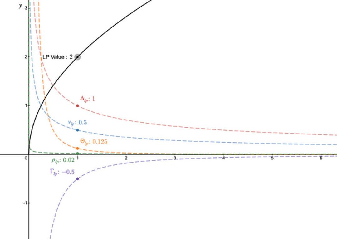
Interactive desmos file for v2: https://www.desmos.com/calculator/inwy6djhhm
Note that, compared to options, Uniswap’s Greek parameters tend to infinity when the price of LP positions falls, as shown by the dashed line at x = 0 in the figure above. To cut these tail risks, we can use the concentration range in v3.
Greek Parameters - Concentrated LP Range v3
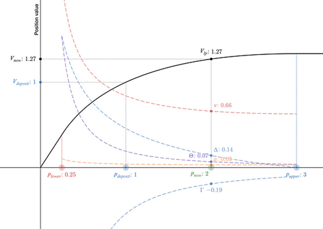
Desmos file for univ3 Greek parameters: https://www.desmos.com/calculator/l8sqzlwkf5
The smaller we focus the range p_a (lower bound) ~ p_b (upper bound), the more sensitive our Delta Δ and Gamma Γ become, note that Gamma is negative, which means our LP payments have a concave black shape. Our theta /Θ / expected fees also increase, while the interest rate sensitivity ρ is largely unaffected.
However, while the payoff graph of a single LP position may match that of an option, the other Greeks may not.
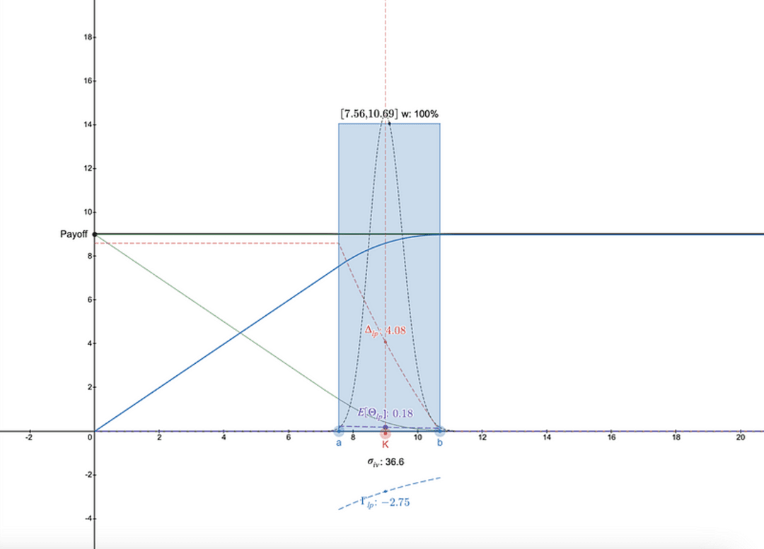
LP Greek parameters do not look like regular options: https://www.desmos.com/calculator/nyuw7sybin
Here, we have a single LP-wide call option, but the other Greeks are not fixed.
The trick that can be used is that instead of trying to find a way to hedge LP positions, one first needs to find an option in the market with a strike price (K) as well as an implied volatility (σ_iv) and an expiration time (t). After that, a series of LP positions can be constructed that follow a lognormal distribution, originally inspired by Dan Robinson's normally distributed liquidity fingerprint for Uniswap v3 [1]. Granularizing LP positions to match a lognormal distribution over price space allows for smoothing of the Greek parameters:
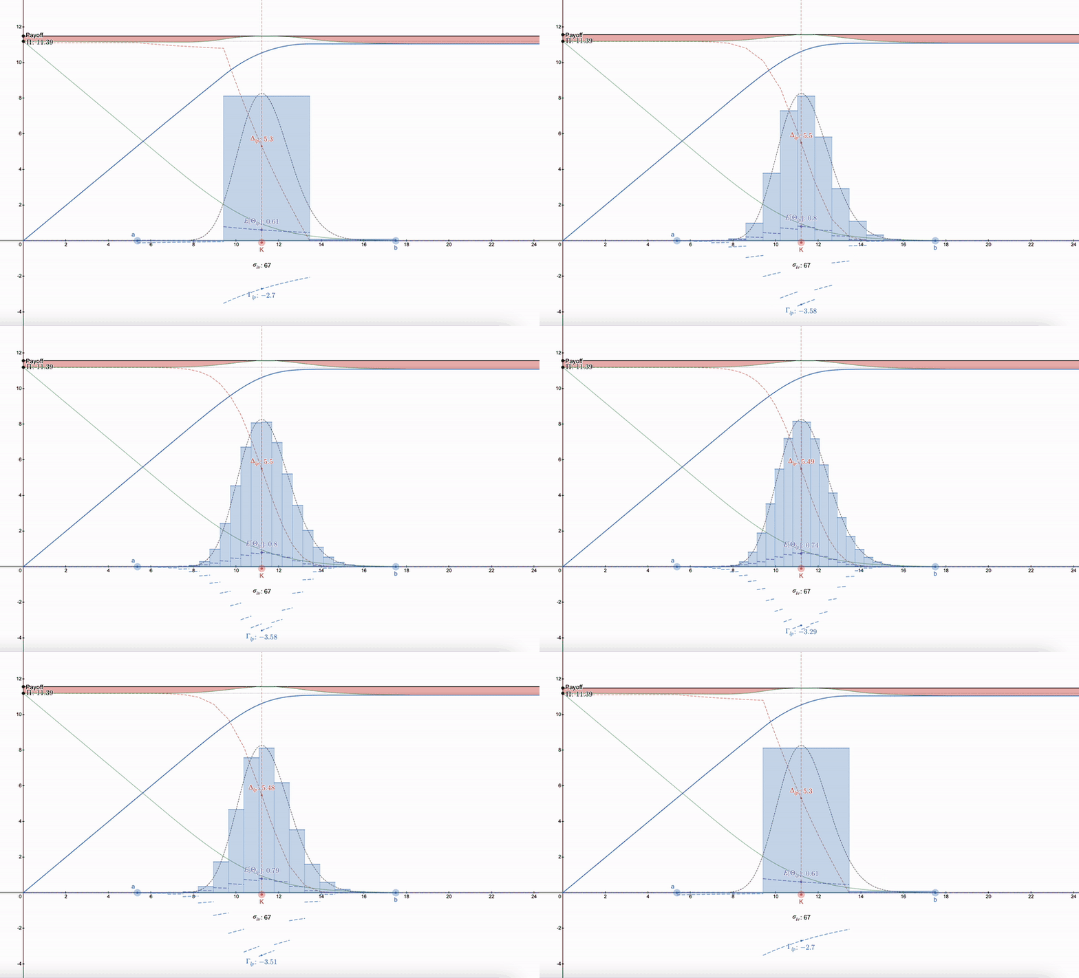
Note that the LP Greeks start to resemble options. Diversification of LP positions allows one to switch to the next range as prices fall. More than 7 LP positions have diminishing returns.
Oddly, it seems very difficult to 100% eliminate the payout using a lognormal distribution (correct me if I’m wrong), but if the lognormal liquidity fingerprint approximates the Dirac Delta function, the above differences (visualized in red in the figure above) disappear. For example, Asian options happen to also follow a lognormal distribution, but surprisingly, they are more price sensitive, with Δ and Γ being sharper, because Asian options have a volatility of 1/√3 of that of regular options, and therefore have less impact on payout divergence:
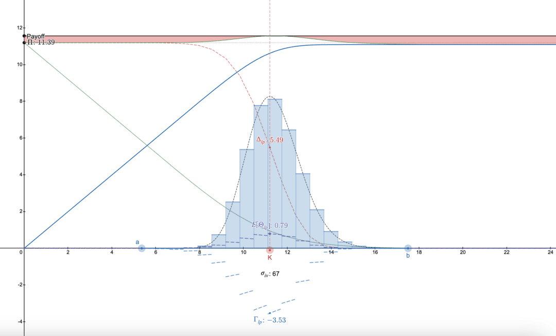
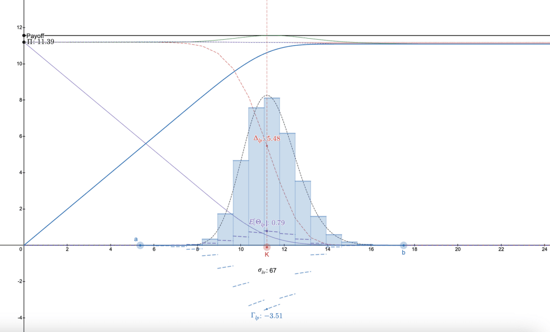
Hedging a portfolio of LP positions using European put options is done by hedging with their equivalent Asian put options.
A single LP position can roughly match a European option but ignore the smoothing Greeks, while a series of LP positions will smooth the Greeks but leave a hill. This tradeoff may be improved in the future with potential adjustments/skewed liquidity fingerprints.
LP Hedging Strategy
On the other hand, if one is not interested in trying to undo concave LP payments, then the desmos file: https://www.desmos.com/calculator/khvbqzncg9. can also be used to see how various payment methods work. Below is an example of a possible series of payments.
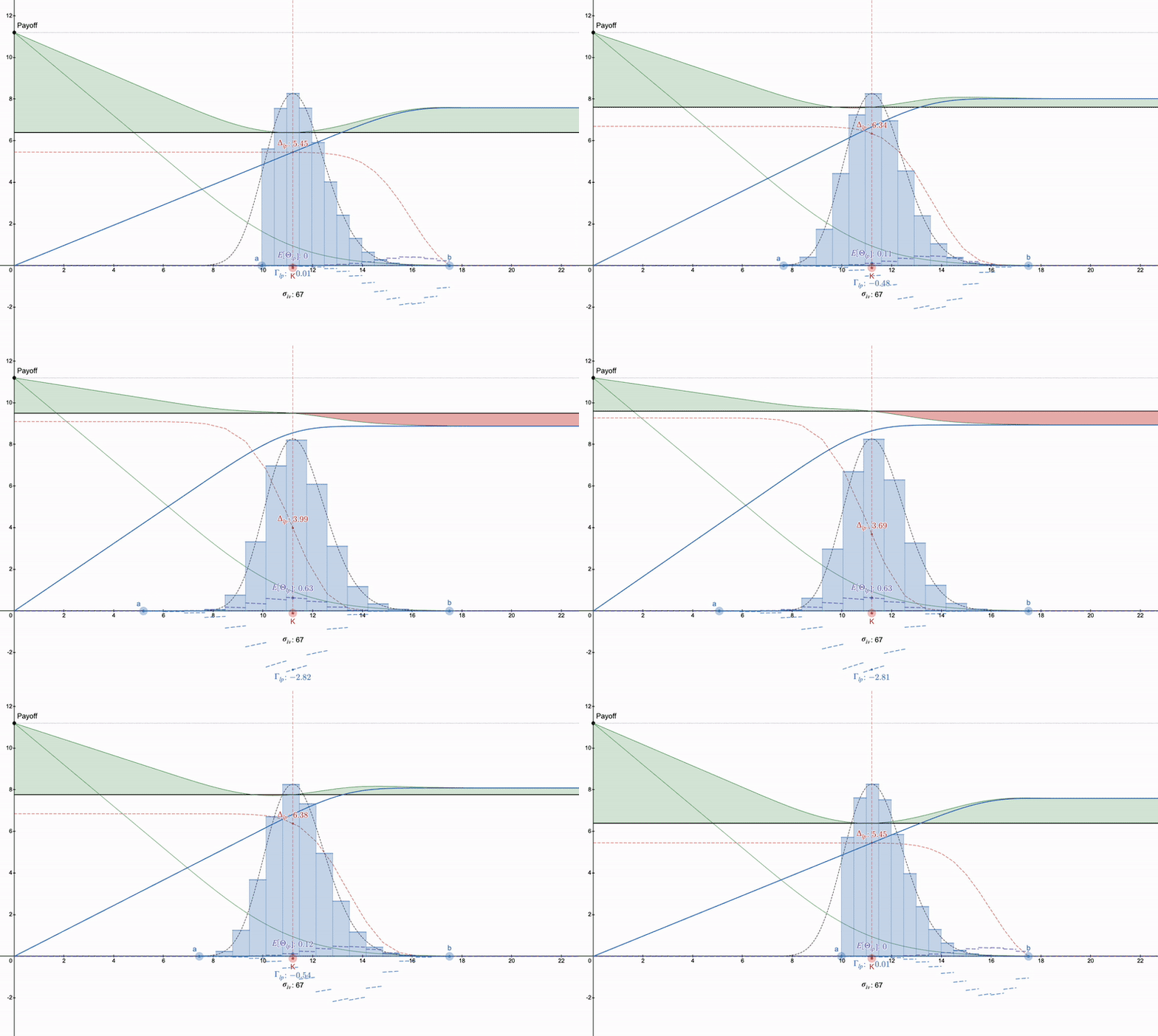
Vertical put spread >> put option >> some kind of long straddle. Note that the put option will compound over time due to theta decay, while the LP position can grow due to fees.
One interesting property of v3 I noticed is that if you concentrate liquidity on p_a at exactly 75% of the current price or less, and set p_b to the current price, then the value of asset X will peak at 25%, which may have some strategic value for someone trying to accumulate the asset.
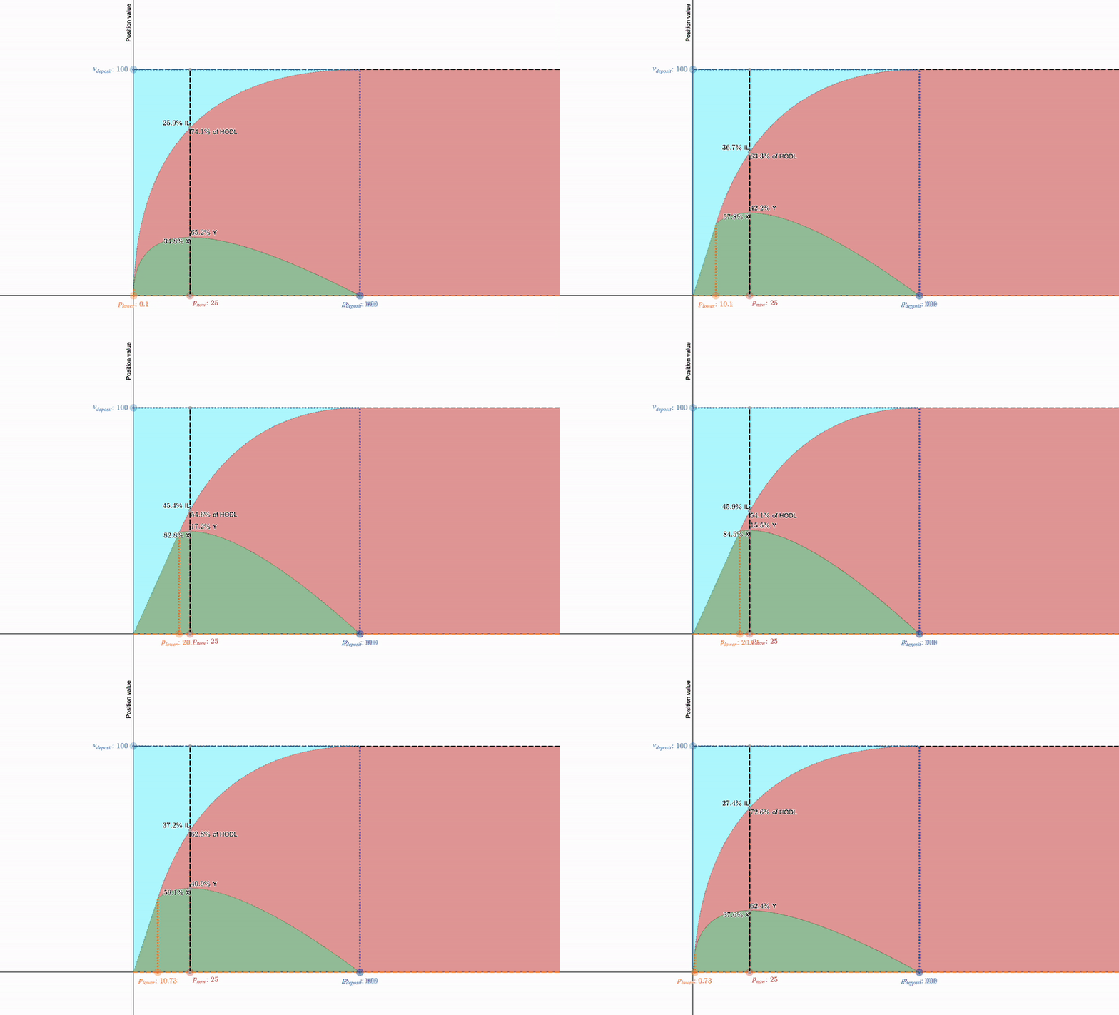
Dan Robinson's v3 tool: https://twitter.com/danrobinson/status/1430678225945042945
A single range like this can be combined with a market put option to get the following payout: https://www.desmos.com/calculator/a8y3pl3t03:
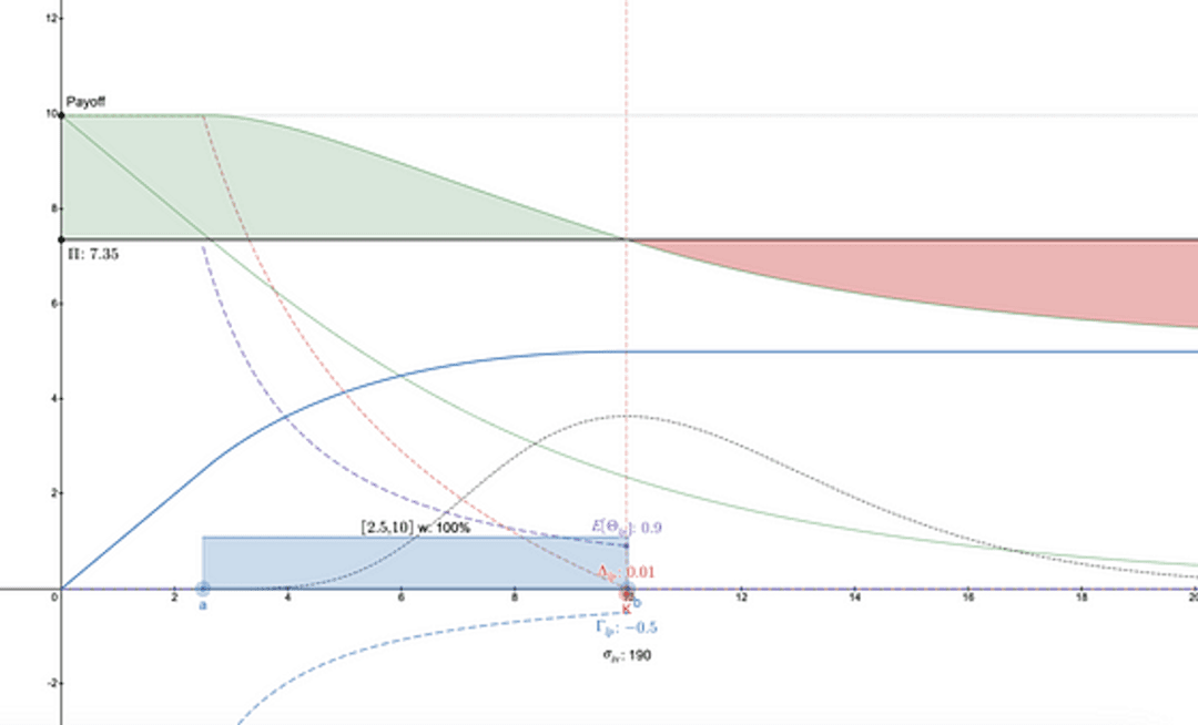
Put option parameters can be extracted from the market. Over time, if prices do not decrease fast enough, the value of the option will decrease.
Such a strategy essentially seeks to buy into a price decline in order to accumulate assets in the future and earn fees. It is important to note that without options, this becomes a much riskier approach and only makes sense if the executor has a very strong belief that the asset will rebound. However, please note that this does not constitute any financial advice, I am just doing the math.
A deeper historical dig leads to LVR:
In Part 4, I pointed out the relationship between the concavity of LP positions and returns, and wanted to expand on this from a historical and LP divergence loss/loss and rebalancing (LVR) perspective.
Taleb notes that the first person to write about the nonlinear relationship between risk and return was Louis Bachelier [2] in his Theory de la Speculation in 1900 [3], attributing it to its similarity to Fourier’s heat equation. Coincidentally, Lambert used the Feynman-Kac approach to solve for the value of concentrated LP positions [4].
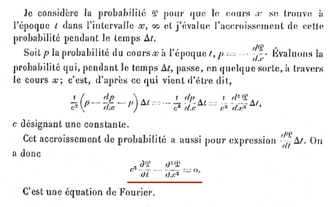
Page 46 of Theory de la Speculation. A constant squared, a dt and a dx²!
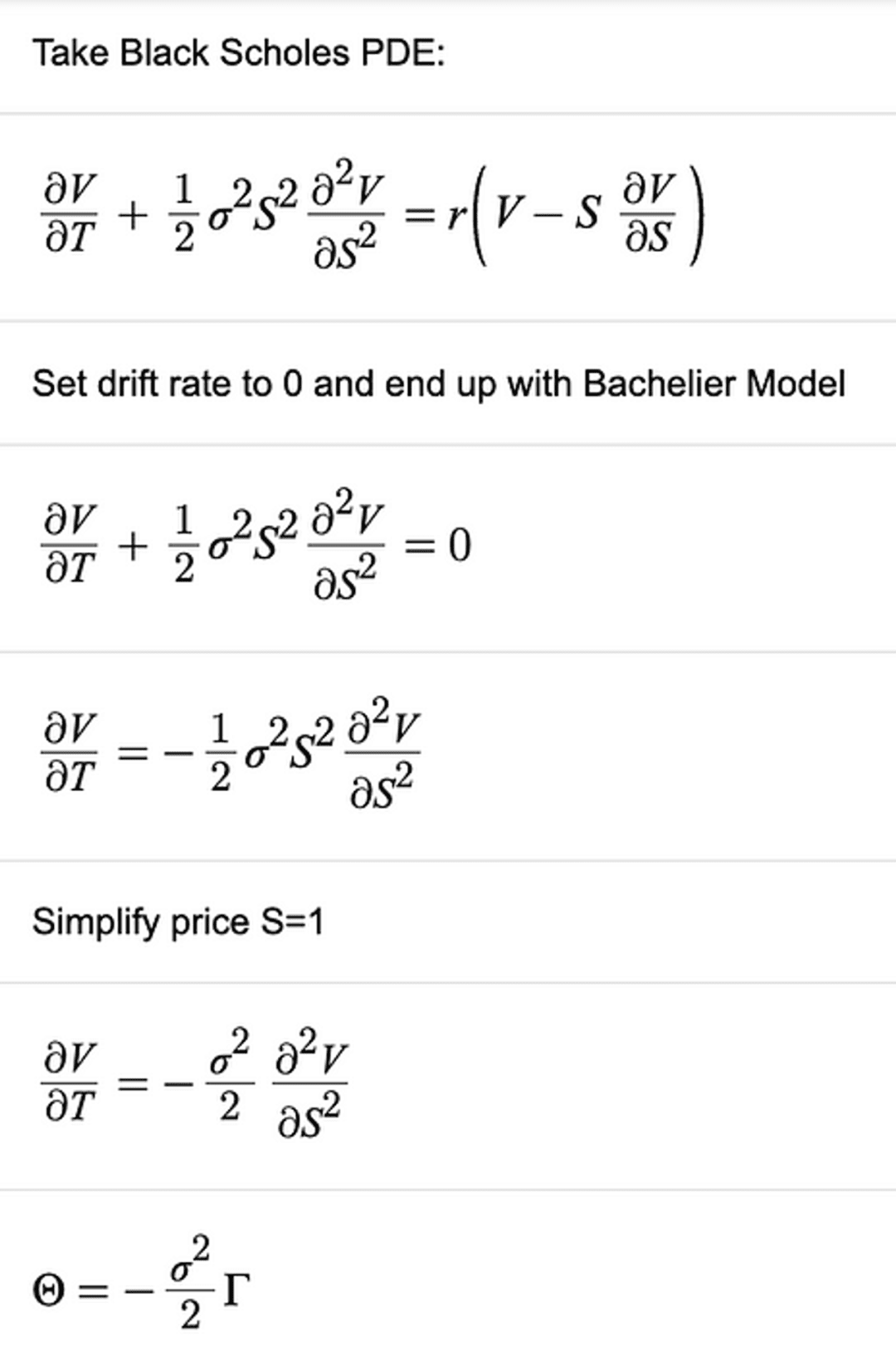
Bachelier's equation is just a slightly rearranged Black-Scholes-Merton equation with the drift rate set to zero.[5]
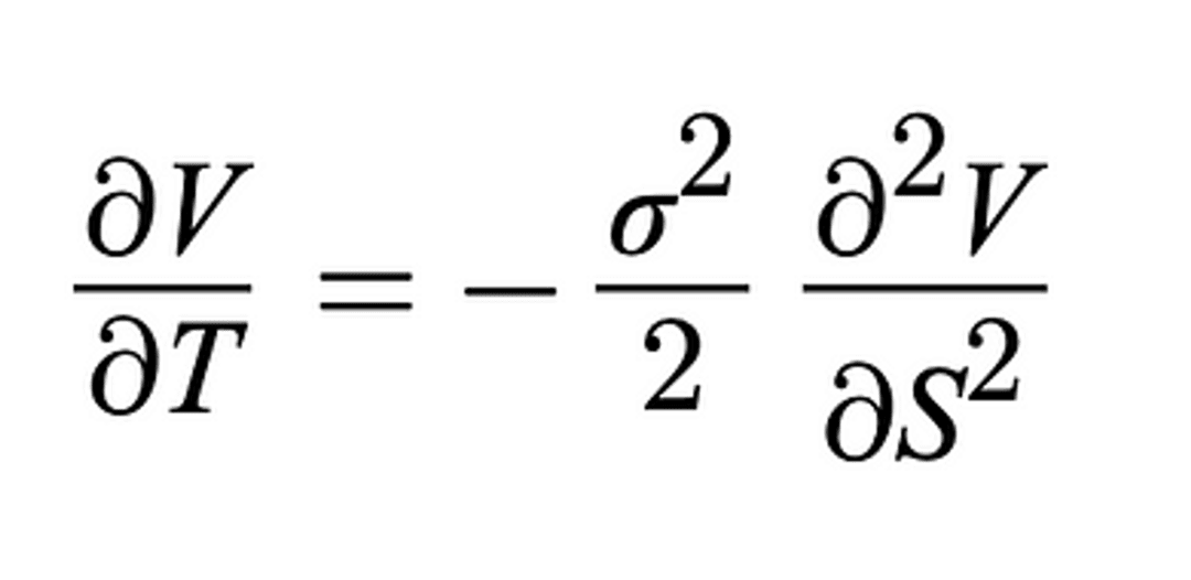
The change in asset prices over time is related to volatility and curvature.
The LHS is theta-Θ, and the RHS is the curvature gamma Γ, which happens to be concave due to the negative sign. Then, Angeris, Evans, and Chitra [6] show that the LP positions of an AMM must have concave payoff functions. From Curve’s CSMM [7] to the entire space of symmetric liquidity curves from Forgy & Lau [8], all LPs should be concave.
By the concave equality in our right-hand side equation, this means that the market maker (LP) position itself must have a premium. If there is no premium, the equality below is violated, and a perpetual long straddle can be constructed by simply borrowing such a LP position and buying part of the underlying asset, waiting for an increase in volatility to exploit it.
Bachelier Equivalence / BSM Dynamic Hedging - Concave commands benefits, while convex commands costs. Mathematically:
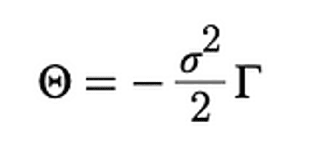
Return ∝ risk times concavity (negative convexity). Derivation of BK in the Appendix.
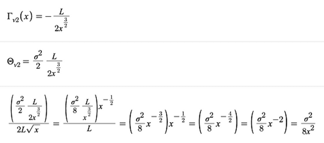
When solving the Theta Greeks for Uniswap[9], I noticed that by substituting the second-order derivative of the LP position into the above formula, I get the same equation as LVR[10].
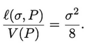
Equation 16. The same result is obtained if Gamma in the Bachelier equivalent is -L/2sqrt(x)³.
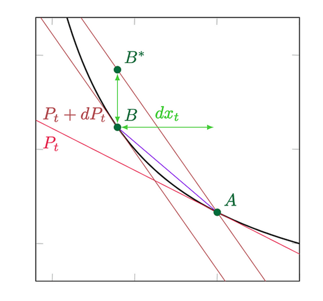
LVR Paper Figure 2 derives the vol²/8 LVR relationship from the above invariant xy=k diagram, which results in a concave LP return.
It is no coincidence that people coming from different perspectives have reached the same conclusion. Lambert actually includes the drift rate[11], while others exclude it[12].
Note that all of these models assume Gaussian distributions, originally derived from Brownian motion (BM) in Ito’s lemma [13], which gives us the internal -σ²/2 term that also appears in the final equation of Angeris, Evans, and Chitra [6], but we know that digital assets, including stablecoins, exhibit Hurst exponents > 0.5, suggesting fractal BM behavior [14], and Sepp and Rakhmonov also showed that stochastic volatility methods are applicable to the skewed implied volatility structure of digital assets [15].
We also see a non-Gaussian tail by examining the tails of the log-log histogram of returns for the most persistent digital assets.
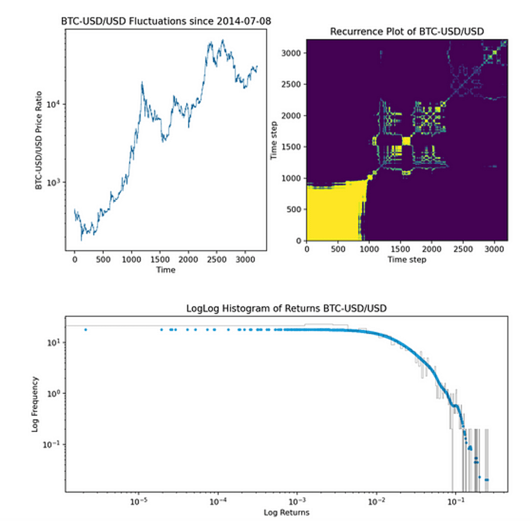
Kernel density smoothing of BTC-USD histogram returns shown in blue
Given the shape of the histogram, we will have to delve into the full range of Uniswap v2 uniform distributions and beyond the Gaussian cliff to gain insight into the appropriate leverage ratio (LVR) theta for market makers.
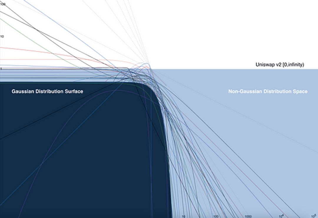
50+ Logarithms of Distributions - Logarithmic Histograms. Exponential and power laws await us in the abyss.
appendix:
Bachelier equivalence derivation.
LVR of Uniswap LP positions derived from the Bachelier equivalent.
References:
https://www.desmos.com/calculator/l1oivvaptt
https://www.maths.usyd.edu.au/u/UG/SM/MATH3075/r/Haug_Taleb_2010.pdf
https://en.wikipedia.org/wiki/Louis_Bachelier#CITEREFBachelier1900a
https://lambert-guillaume.medium.com/pricing-uniswap-v3-lp-positions-towards-a-new-options-paradigm-dce3e3b50125
https://en.wikipedia.org/wiki/Black%E2%80%93Scholes_equation
https://arxiv.org/abs/2103.14769
https://classic.curve.fi/files/stableswap-paper.pdf
https://arxiv.org/pdf/2111.08115.pdf
https://www.desmos.com/calculator/fg8a730ddz
https://arxiv.org/pdf/2208.06046.pdf
https://lambert-guillaume.medium.com/an-analysis-of-the-expected-value-of-the-impermanent-loss-in-uniswap-bfbfebbefed2
https://twitter.com/odtorson/status/1603337199465865216?s=46&t=e0EQ5vcj_HihnkeZ26T4eA
https://en.wikipedia.org/wiki/It%C3%B4%27s_lemma#Geometric_Brownian_motion
https://scholar.google.com/scholar?q=modelling+multifractal+properties+of+cryptocurrency+markets&hl=en&as_sdt=0&as_vis=1&oi=scholart
https://papers.ssrn.com/sol3/papers.cfm?abstract_id=2810768