V moderní finanční teorii hodnocení výkonnosti investic často přesahuje tradiční analýzu průměrného výnosu a standardní odchylky. Zatímco etablované metriky jako Sharpeho poměr se spoléhají na předpoklad normálního rozdělení výnosů, data z reálného trhu—zejména pro digitální aktiva jako Bitcoin (BTC)—často vykazují asymetrii a "tlusté ocasy." Omega poměr nabízí zásadně odlišný přístup využitím celého kumulativního rozdělení výnosů k rozlišení potenciálu zisku od rizika ztráty vzhledem k definovanému prahu.
1. Definice a matematický základ
Podle výzkumu Kapsos et al. (2011) Omega poměr umožňuje analytikům hodnotit pravděpodobnost dosažení konkrétního cílového výnosu integrací celé pravděpodobnostní hustoty. Poměr je definován jako vztah mezi pravděpodobnostně váženými zisky a pravděpodobnostně váženými ztrátami na prahu minimální akceptovatelné návratnosti (MAR).
Matematická reprezentace Omega (Ω) je odvozena prostřednictvím kumulativní distribuční funkce (CDF):

Kde:
Ω: Omega poměr.
𝞃 (tau): Minimální akceptovatelná návratnost (MAR) definovaná investorem.
F(r): Kumulativní distribuční funkce (CDF) návratnosti aktiva.
r: Návratnost aktiva.
Integrací podle částí lze rovnici prezentovat v computačně aplikovatelné podobě založené na očekávaných hodnotách. To určuje hmotnost rozdělení návratnosti nad prahem [𝞃, +∞] (pozitivní návratnost vzhledem k 𝞃) a pod prahem [-∞, 𝞃] (negativní návratnost vzhledem k 𝞃):

Kde:
E[(r - 𝞃)+]: Očekávaná hodnota zisků nad prahem 𝞃.
E[(𝞃 - r)+]: Očekávaná hodnota ztrát pod prahem 𝞃.
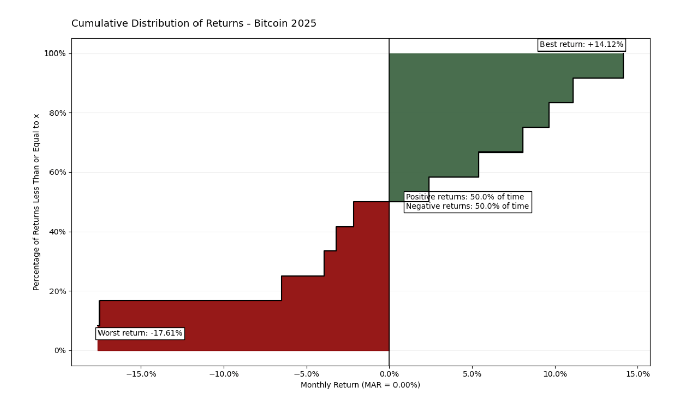
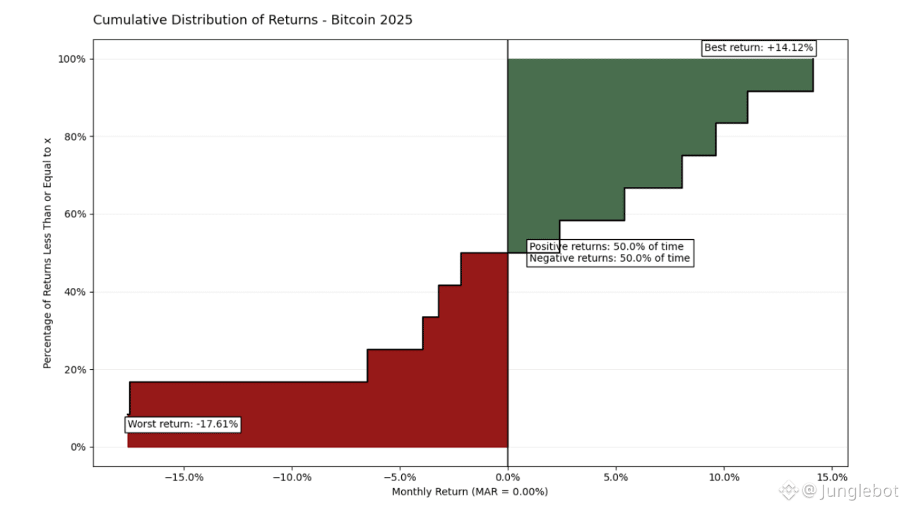
Data z roku 2025 ilustrují asymetrickou volatilitu aktiva, s extrémními výkyvy pohybujícími se mezi -17,61 % a +14,12 %. Přestože je frekvence vyvážená (50 % pozitivních vs. 50 % negativních měsíců), Omega poměr 0,778 odhaluje těžší váhu ztrát v levém ocase křivky. Tato vizuální parita zdůrazňuje, že velikost poklesů dominuje rallyům, což slouží jako základní základ pro hodnocení kvality aktiva vzhledem k zvolenému MAR.
Zatímco roční graf se může zdát objemný a méně informativní, rozšíření časového horizontu na 10letou periodu poskytuje výrazně komplexnější obraz.
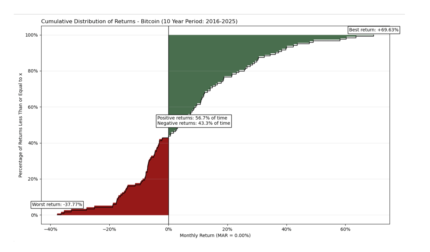
Desetiletá analýza odhaluje mnohem příznivější profil rizika a výnosu. I když aktivum zachovává extrémní volatilitu s měsíčními poklesy až -37,77 %, vykazuje impozantní růstový potenciál s vrcholy až +69,63 %. Na rozdíl od ročního snímku zde dominují pozitivní měsíce (56,7 % času) a "zelená zóna" zisku vizuálně i matematicky převyšuje "červenou zónu" rizika. Omega poměr pro toto období je 1,621, což dokazuje, že Bitcoin generuje významný prémium vzhledem k riziku, které je podstoupeno v dlouhém období.
2. Interpretace a analýza rizika
Na rozdíl od jiných koeficientů závisí hodnota Omega přímo na zvoleném prahu 𝞃. To činí metriku adaptivní na specifický rizikový profil investora.
Ω > 1: Naznačuje, že kumulativní hodnota zisků převyšuje hodnotu ztrát vzhledem k zvolenému MAR. Vyšší číslo znamená lepší kvalitu výnosů.
Ω = 1: Znamená to, že očekávaný výnos aktiva je přesně roven prahu 𝞃.
Ω < 1: Signalizuje, že riziko ztráty pod zvolenou "barierou" převyšuje potenciál pro zisk.
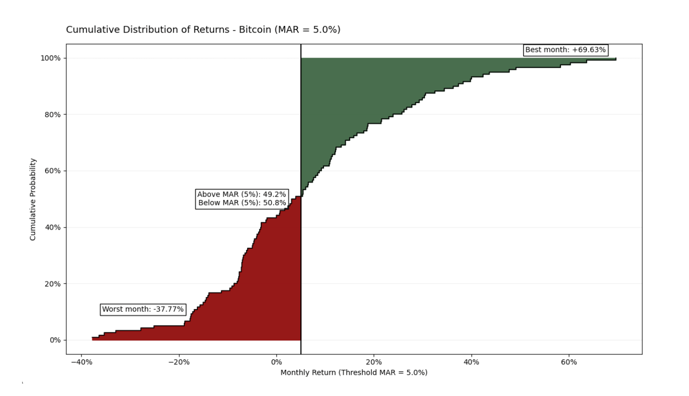
V analyzovaném desetiletém období umístění MAR 5 % měsíčně staví aktivum do přísnějšího rámce. I když Bitcoin zůstává pod tímto prahem 50,8 % času, jeho Omega poměr zůstává pozitivní na 1,2102. To potvrzuje, že přínos "explozivních" měsíců (dosahujících až +69,63 %) je dostatečně silný na to, aby převážil kumulativní efekt měsíců se zápornými nebo průměrnými výnosy. Data dokazují, že i při vysokých investičních očekáváních si Bitcoin udržuje svou statistickou výhodu v dlouhém období.
3. Optimalizace pomocí lineárního programování
Jednou z nejvýznamnějších praktických aplikací Omega poměru, podrobně uvedenou Kapsos et al. (2011), je jeho využití při aktivní konstrukci portfolia. Zatímco funkce se může zpočátku zdát složitá na výpočet, autoři dokládají, že maximalizace Omega může být přeformulována jako problém lineárního programování.
Diskrétní analog Omega pro výpočetní účely na základě $m$ historických pozorování je:

Kde:
𝑤: Vektor váh aktiv v portfoliu.
r: Vektor historických průměrných výnosů.
m: Počet historických pozorování (vzorků).
rj: Vektor výnosů pro každé konkrétní pozorování ⅉ.
Tento přístup je zásadně odlišný od tradiční optimalizace Markowitze (průměr-varianta). Místo toho, aby se prostě minimalizovala volatilita (což penalizuje ostré vzestupy), Omega model umožňuje investorům do Bitcoinu optimalizovat své pozice tak, aby maximalizovali "horní ocas" rozdělení. Přidáním jedné k poměru čistého nadměrného výnosu k průměrnému nedostatku, Kapsosova formule umožňuje algoritmům rychle a efektivně najít váhy (𝑤), které nabízejí nejlepší pravděpodobnost úspěchu vzhledem k cílům jednotlivých investorů.
4. Komparativní analýza: Bitcoin vs. S&P 500
Abychom porozuměli skutečné hodnotě Omega poměru, je nutné porovnat Bitcoin s tradičním benchmarkem, jako je index S&P 500. Tradiční metriky rizika jako standardní odchylka často selhávají, protože nezohledňují asymetrii a rozdíly ve "struktuře ocasu" obou rozdělení.
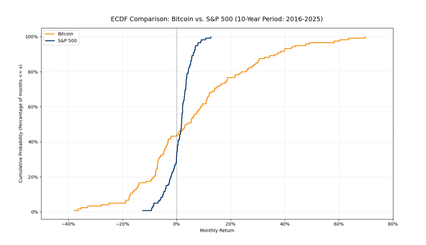
Tento komparativní graf ECDF ilustruje zásadní rozdíl mezi dvěma aktivy:
Koncentrace vs. volatilita: Čára S&P 500 (tmavě modrá) je výrazně strmější a soustředěná v úzkém rozmezí kolem nuly. To značí aktivum s nižší volatilitou a těsnějším, předvídatelnějším rozdělením.
Bitcoinovy "tlusté ocasy": Čára Bitcoinu (oranžová) vykazuje výrazně širší extrémy. To je vizuální důkaz "tlustých ocasů"—vyšší pravděpodobnost obrovských negativních a pozitivních odchylek ve srovnání s tradičním trhem.
Specifika výkonu: Zatímco nejhorší měsíc Bitcoinu dosáhl -37,77 %, aktivum úspěšně generovalo explozivní růstové období až +69,63 %. Tyto asymetrické skoky v "pravém ocase" jsou důvodem, proč Bitcoin často generuje mnohem vyšší Omega poměr při nižších úrovních MAR.
Závěr: Srovnání potvrzuje, že Omega je spravedlivější metrika rizika než standardní odchylka. Uznává vysoký potenciál Bitcoinu, aniž by ignorovalo jeho charakteristiky "tlustého ocasu", zatímco umožňuje investorům aplikovat optimalizační vzorec k vyvážení váh portfolia (𝑤) vůči požadovanému prahovému výnosu (𝞃).
Závěrečná závěr
Analýza pomocí Omega poměru dokazuje, že tradiční metriky jako Sharpeho poměr jsou nedostatečné pro aktiva s "tlustými ocasy" jako Bitcoin. Zatímco jeden rok může být zavádějící, desetiletý horizont odhaluje statistickou dominanci zisků (Ω = 1,621). I při vysokém prahu MAR = 5 % si aktivum udržuje svou efektivitu (Ω = 1,2102) díky velikosti svých pozitivních odchylek. Srovnání se S&P 500 zdůrazňuje, že Bitcoin nabízí jedinečné vystavení "pravému ocasu" rozdělení. Využití modelu Kapsos et al. transformuje tyto teoretické poznatky do praktického nástroje pro optimalizaci portfolia pomocí lineárního programování. Nakonec Omega poměr poskytuje poctivější a adaptivní hodnocení rizika, uznávající potenciál pro explozivní růst.
Reference
Kapsos, M., Zymler, S., Christofides, N., a Rustem, B. (2011). Optimalizace Omega poměru pomocí lineárního programování. Imperial College London.